Performance profiling of some of the eBay code base showed the logarithm (log) function to be consuming more CPU than expected. The implementation of log in modern math libraries is an ingenious wonder, efficiently computing a value that is correct down to the last bit. But for many applications, you’d be perfectly happy with an approximate logarithm, accurate to (say) 10 bits, especially if it were two or three times faster than the math library version. This post is the first of a series that examines approximate logarithms and the tradeoff between accuracy and speed. By the end of the series, you will see how to design fast log functions, and will discover that on a MacBook Pro, you can get a roughly 3x speedup if you are willing to settle for 7 bits. Alternatively, if you want more accuracy you can get 11 bits with a 2x speedup. The numbers might vary for your target machine, but I will present code so that you can determine the tradeoffs for your case.
You can find code for approximate logs on the web, but they rarely come with an evaluation of how they compare to the alternatives, or in what sense they might be optimal. That is the gap I’m trying to fill here. The first post in this series covers the basics, but even if you are familiar with this subject I think you will find some interesting nuggets. The second post considers rounding error, and the final post gives the code for a family of fast log functions.
A very common way to to compute log (meaning  ) is by using the formula
  to reduce the problem to computing
  . The reason is that for arbitrary
  is easily reduced to the computation of
  for in the interval
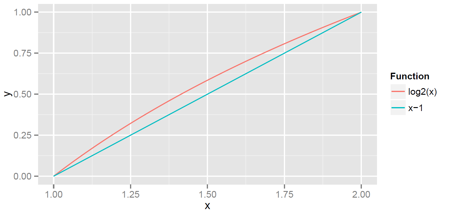
  ; details below. So for the rest of this series I will exclusively focus on computing . The red curve in the plot below shows on
 ![[1, 2]](assets/Uploads/Blog/Imported/quicklatex.com-31ff03a000843062dd81e31e15f9f923_l3.svg "Rendered by QuickLaTeX.com") . For comparison, I also plot the straight line
. For comparison, I also plot the straight line  .
.
If you’ve taken a calculus course, you know that  has a Taylor series about
  which is
  . Combining with
  gives (
 for Taylor)
![\[ t(x) \approx -0.7213 x^2 + 2.8854 x - 2.1640 \]](assets/Uploads/Blog/Imported/quicklatex.com-fb051feb9113d6b34929aa52b37edbb4_l3.svg "Rendered by QuickLaTeX.com")
How well does  approximate ?
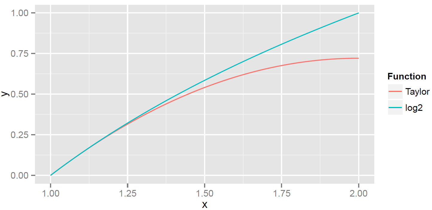
The plot shows that the approximation is very good when  , but is lousy for near 2—so is a flop over the whole interval from 1 to 2. But there is a function that does very well over the whole interval:
  . I call it
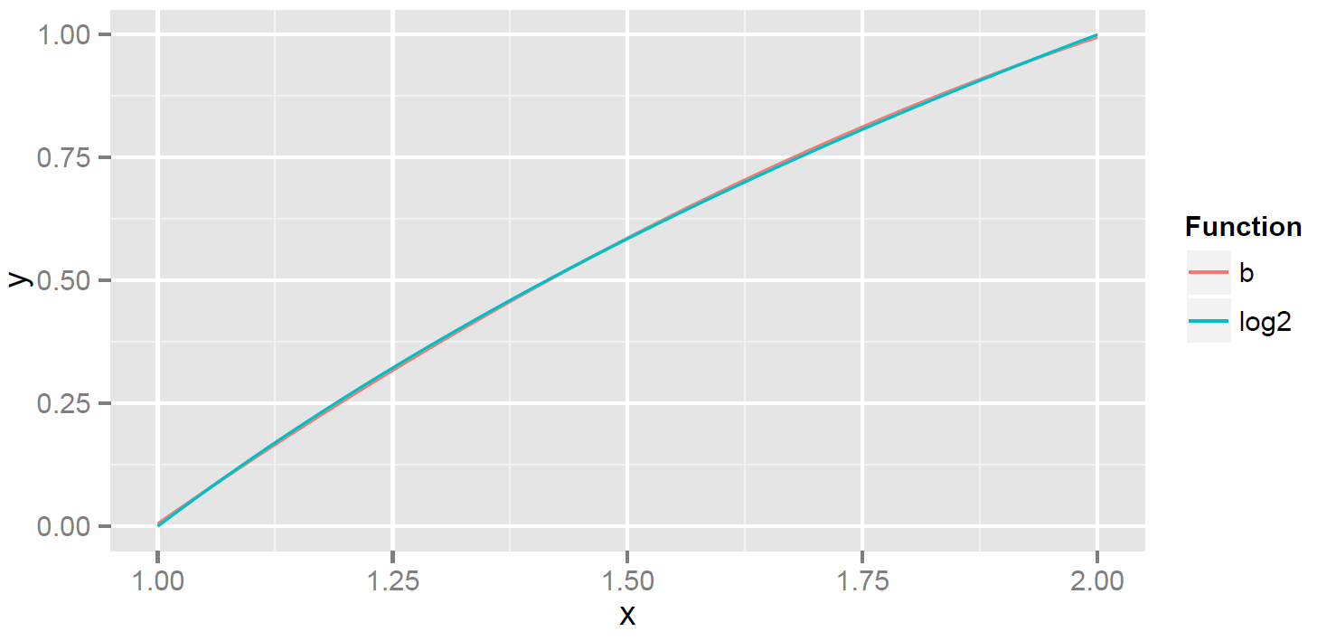
  for better. It is shown below in red ( in blue). The plot makes it look like a very good approximation.
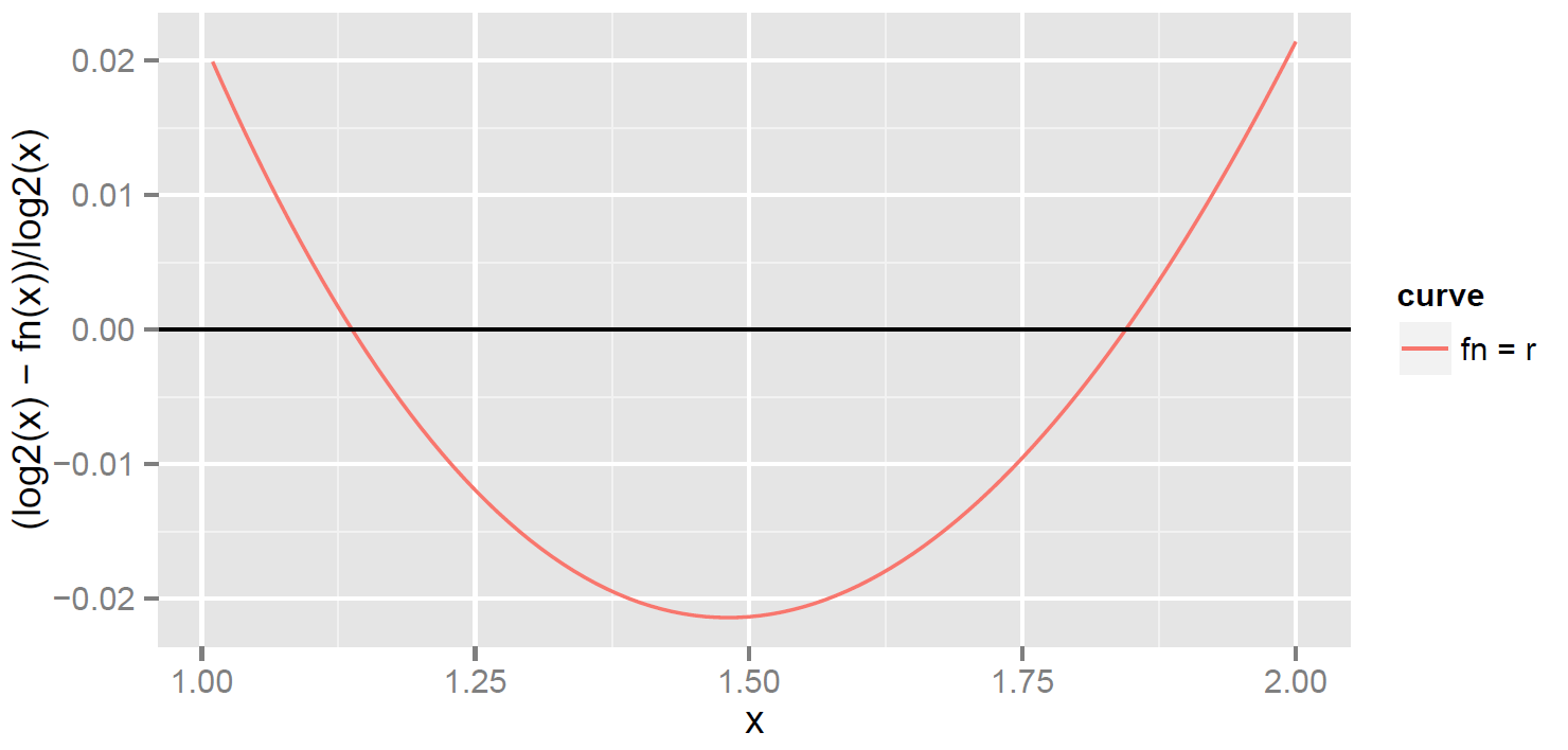
A better way to see quality of the approximation is to plot the error  . The largest errors are around
  and
and  .
.
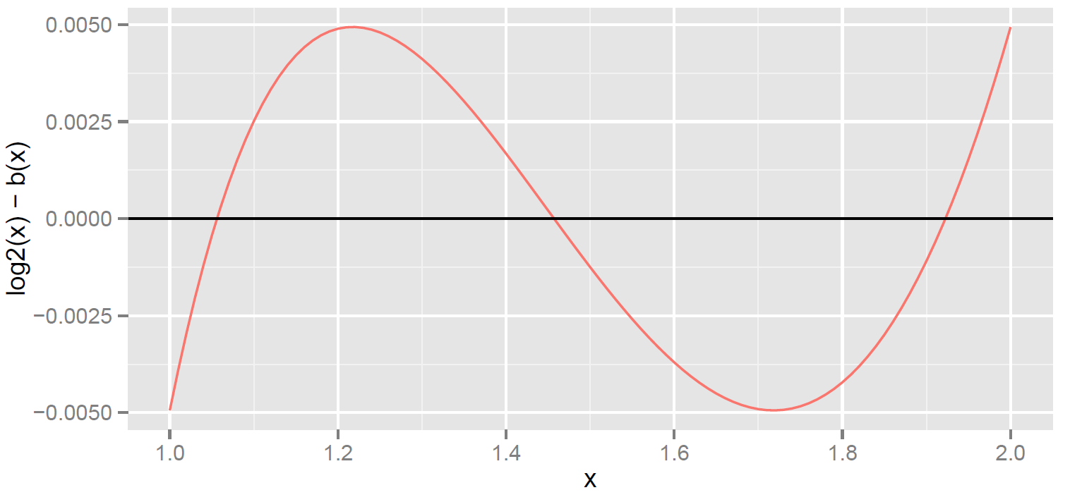
Now that I’ve shown you an example, let me get to the first main topic: how do you evaluate different approximations? The conventional answer is minimax. Minimax is very conservative—it only cares about the worst (max) error. It judges the approximation over the entire range  by its error on the worst point. As previously mentioned, in the example above the worst error occurs at , or perhaps at , since the two have very similar errors. The term minimax means you want to minimize the max error, in other words find the function with the minimum max error. The max error here is very close to 0.0050, and it is the smallest you can get with a quadratic polynomial. In other words, solves the minimax problem.
Now, onto the first of the nuggets mentioned at the opening. One of the most basic facts about  is that
  , whether it’s or
  or
or  . This means there’s a big difference between ordinary and relative error when .
As an example, take  . The error in is quite small:
  . But most likely you care much more about relative error:
  , which is huge, about
  . It’s relative error that tells you how many bits are correct. If
  and
and  agree to
  bits, then is about
  . Or putting it another way, if the relative error is
  , then the approxmation is good to about
  bits.
bits.
The function that solved the minimax problem solved it for ordinary error. But it is a lousy choice for relative error. The reason is that its ordinary error is about  near . As
  it follows that
  , and so the relative error will be roughly
  . But no problem. I can compute a minimax polynomial with respect to relative error; I’ll call it
  for relative. The following table compares the coefficients of the Taylor method , minimax for ordinary error and minimax for relative error
  :
:

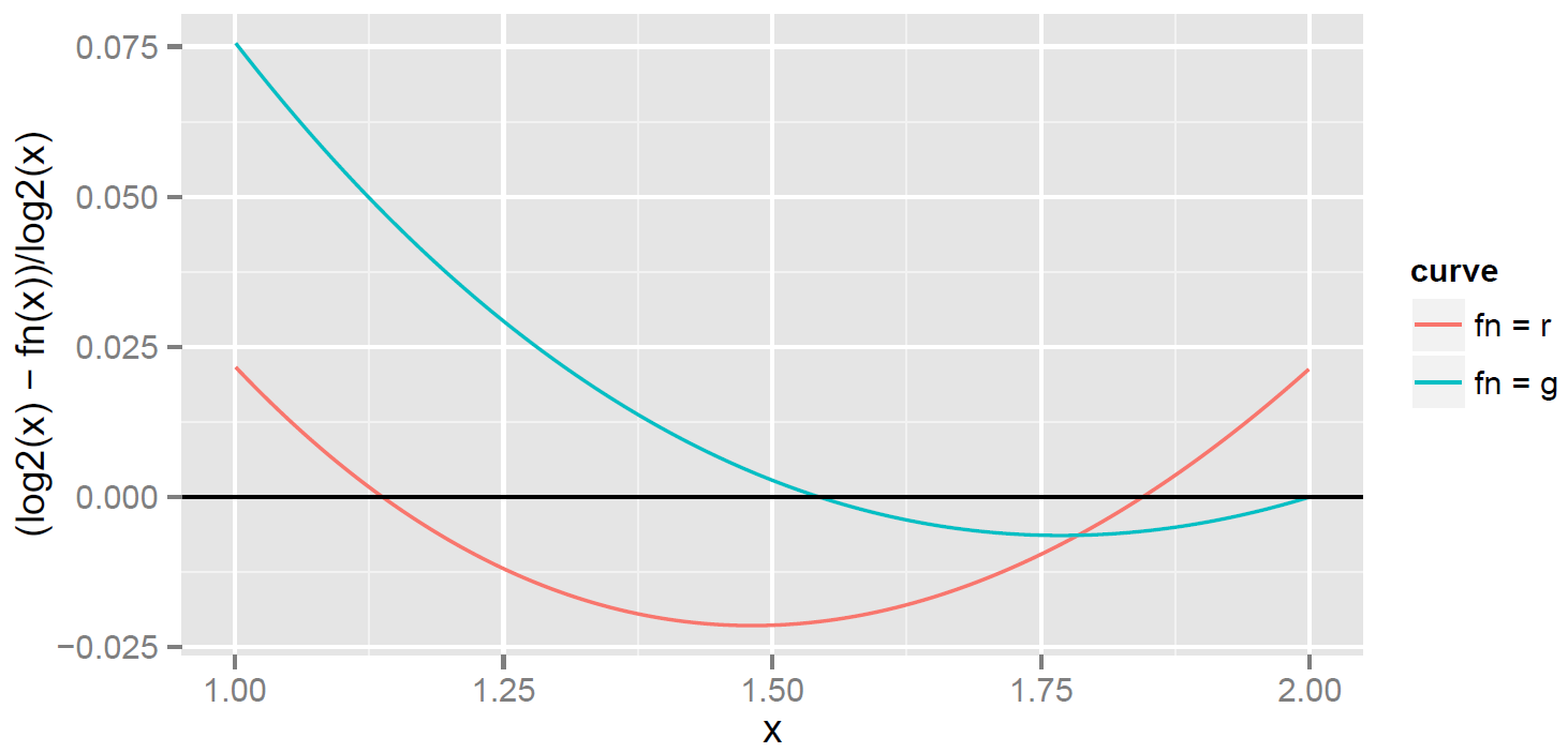
The coefficients of and are similar, at least compared to , but is a function that is always good to at least 5 bits, as the plot of relative error (below) shows.
Here’s a justification for my claim that is good to 5 bits. The max relative error for occurs at ,  , and
, and  . For example, at

 .
.
Unfortunately, there’s a big problem we’ve overlooked. What happens outside the interval [1,2)? Floating-point numbers are represented as  with
with  . This leads to the fact mentioned above:
  . So you only need to compute on the interval
  . When you use for and reduce to this range for other , you get
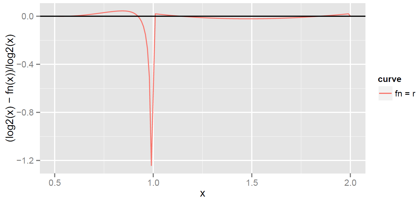
The results are awful for just below 1. After seeing this plot, you can easily figure out the problem. The relative error of for  is about 0.02, and is almost the same as ordinary error (since the denominator is close to
  ). Now take an just below 1. Such an is multiplied by 2 to move it into [1,2), and the approximation to is
  , where the
  compensates for changing to
  . The ordinary error
  is still about 0.02. But is very small for , so the ordinary error of 0.02 is transformed to
  , which is enormous. At the very least, a candidate for small relative error must satisfy
  . But
. But  . This can be fixed by finding the polynomial that solves the minimax problem for all . The result is a polynomial
  for global.

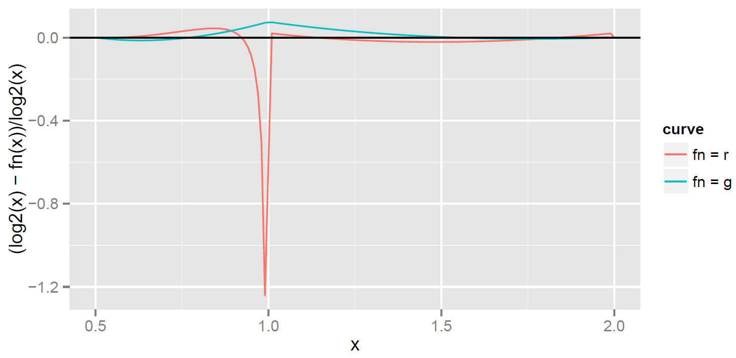
Globally (over all ), the blue curve does dramatically better, but of course it comes at a cost. Its relative error is not as good as over the interval [1, 2). That’s because it’s required to satisfy  in order to have a small relative error at
  . The extra requirement reduces the degrees of freedom, and so does less well on [1, 2].
Finally, I come to the second nugget. The discussion so far suggests rethinking the basic strategy. Why reduce to the interval [1,2)? Any interval  will do. What about using [0.75, 1.5)? It is easy to reduce to this interval (as I show below), and it imposes only a single requirement: that
  . This gives an extra degree of freedom that can be used to do a better job of approximating . I call the function based on reduction [0.75, 1.5)
  for shift, since the interval has been shifted.

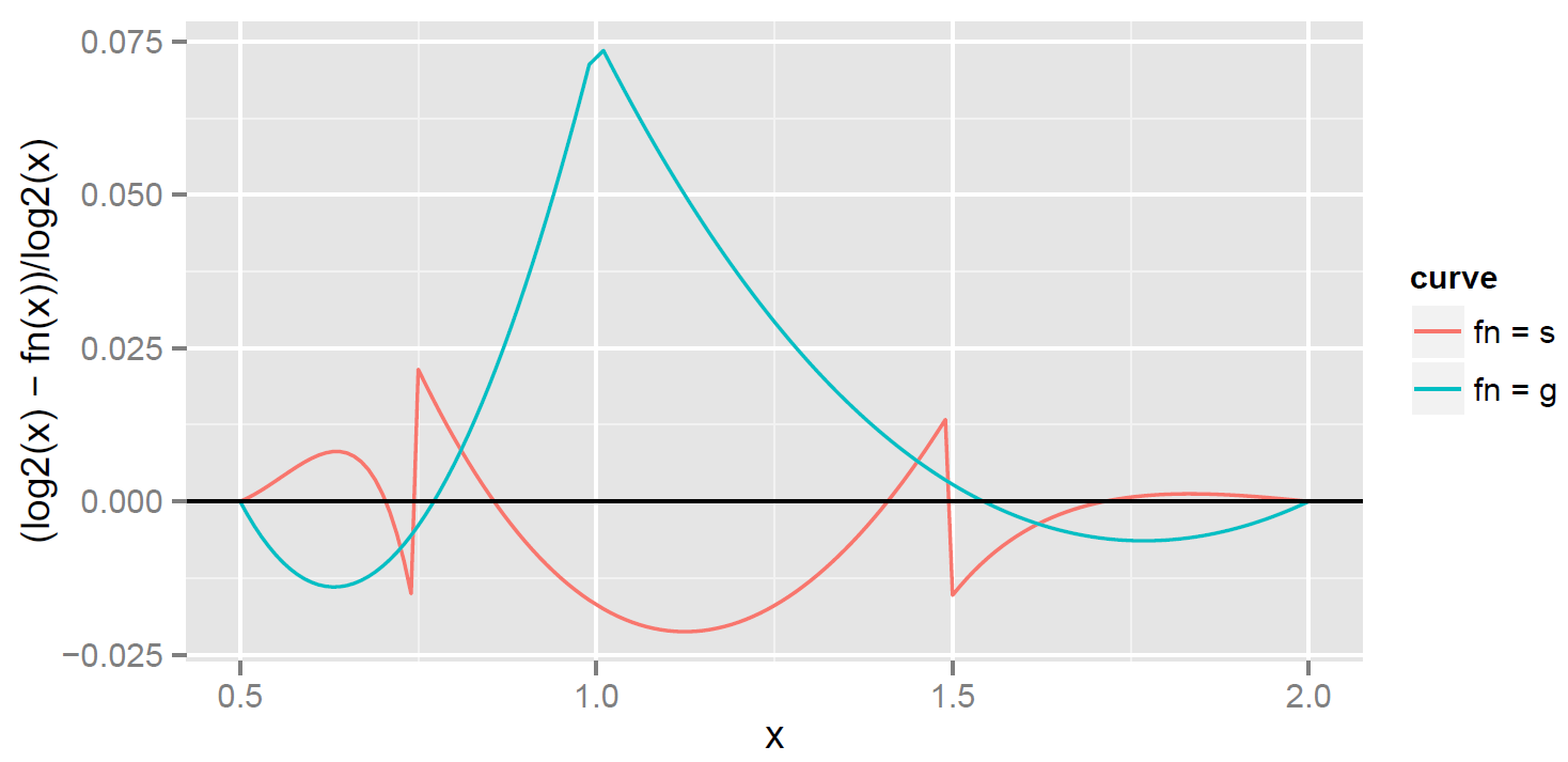
The result is a thing of beauty! The error of is significantly less than the error in . But you might wonder about the cost: isn’t it more expensive to reduce to [0.75, 1.5) instead of [1.0, 2.0)? The answer is that the cost is small. A floating-point number is represented as  , with
  stored in the right-most 23 bits. To reduce to [0.75, 1.5) requires knowing when
  , and that is true exactly when the left-most of the 23 bits is one. In other words, it can be done with a simple bit check, not a floating-point operation.
Here is more detail. To reduce to  , I first need code to reduce to the interval . There are library routines for this of course. But since I’m doing this whole project for speed, I want to be sure I have an efficient reduction, so I write my own. That code combined with the further reduction to is below. Naturally, everything is written in single-precision floating-point. You can see that the extra cost of reducing to [0.75, 1.5) is a bit-wise operation to compute the value
  , and a test to see if is nonzero. Both are integer operations.
The code does not check that  , much less check for infinities or NaNs. This may be appropriate for a fast version of log.
float fastlog2(float x)  // compute log2(x) by reducing x to [0.75, 1.5)
{
    // a*(x-1)^2 + b*(x-1) approximates log2(x) when 0.75 <= x < 1.5
    const float a =  -.6296735;
    const float b =   1.466967;
    float signif, fexp;
    int exp;
    float lg2;
    union { float f; unsigned int i; } ux1, ux2;
    int greater; // really a boolean
    /*
     * Assume IEEE representation, which is sgn(1):exp(8):frac(23)
     * representing (1+frac)*2^(exp-127)  Call 1+frac the significand
     */

    // get exponent
    ux1.f = x;
    exp = (ux1.i & 0x7F800000) >> 23;
    // actual exponent is exp-127, will subtract 127 later

    greater = ux1.i & 0x00400000;  // true if signif > 1.5
    if (greater) {
        // signif >= 1.5 so need to divide by 2.  Accomplish this by
        // stuffing exp = 126 which corresponds to an exponent of -1
        ux2.i = (ux1.i & 0x007FFFFF) | 0x3f000000;
        signif = ux2.f;
        fexp = exp - 126;    // 126 instead of 127 compensates for division by 2
        signif = signif - 1.0;                    // <
        lg2 = fexp + a*signif*signif + b*signif;  // <
    } else {
        // get signif by stuffing exp = 127 which corresponds to an exponent of 0
        ux2.i = (ux1.i & 0x007FFFFF) | 0x3f800000;
        signif = ux2.f;
        fexp = exp - 127;
        signif = signif - 1.0;                    // <<--
        lg2 = fexp + a*signif*signif + b*signif;  // <<--
    }
    // lines marked <<-- are common code, but optimize better
    //  when duplicated, at least when using gcc
    return(lg2);
} with 0x3f000000 in one branch and 0x3f800000 in the other, you can have a single branch that uses
 ![\mathsf{arr[greater]}](assets/Uploads/Blog/Imported/quicklatex.com-da0957f283ff74c30f9776d4eaaf7e04_l3.svg "Rendered by QuickLaTeX.com") . Similarly for the other difference in the branches, exp−126 versus exp−127. This was not faster on my MacBook.
. Similarly for the other difference in the branches, exp−126 versus exp−127. This was not faster on my MacBook.
In summary:
- To study an approximation
 , don’t plot and directly, instead plot their difference.
 - The measure of goodness for is its maximum error.
- The best is the one with the smallest max error (minimax).
- For a function like , ordinary and relative error are quite different. The proper yardstick for the quality of an approximation to is the number of correct bits, which is relative error.
- Computing requires reducing to an interval but you don’t need
 . There are advantages to picking
  instead.
In the next post, I’ll examine rounding error, and how that affects good approximations.
Powered by QuickLaTeX