In our previous article, “Seven Tips for Visual Search at Scale,” we discussed visual search where a user query is an image, and the results are shown to the user based on visual similarity to that query image. One could consider this as a single iteration of the search process. This is great when the user has the picture of the exact product and finds the right match in the result set in terms of price, size, condition, shipping, etc. It is still possible that the exact product is not in the result set for reasons such as product out of stock. What if (i) the user knows the exact product but does not have the picture or (ii) the user has an image of a product but wants one with a few variations from the query or (iii) the user wants to explore the beautiful product landscape? An interactive approach is natural in such scenarios where the user gives feedback after each result set. Such feedback could be based on items in the result set that had a click-through from the search result page. Results on the next (unseen) page could be updated based on images that experienced a click-through. We present an approach for interactive visual search.
Scope
Although the same could be true for text or speech or multimodal search, we limit our discourse to image queries. The aim of this material is to keep it simple. More technical details can be found in our paper “Give me a hint! Navigating Image Databases using Human-in-the-loop Feedback,” that was presented at WACV 2019. Watch the 5-minute video at the end of this article as an alternative. The scope of this article does not include personalization, but includes only user feedback during the search session for a single quest. However, extension to personalization is straightforward, since our approach could be generalized easily.
Background: similarity using triplet embedding
We represent each image by a compact signature in the form of a series of numbers represented as a vector a.k.a. embedding. Similarity is then measured by proximity based on this vector. This is illustrated in Figure 1. This vector could be generated by a deep neural network, i.e. the deep neural network maps the input image to a vector. One way to train such deep neural networks is to train it using triplets and predict if they have the desired order. The resulting embedding is called “triplet embedding.” Valid triplets are constructed such that they are made up of three images (A, P, N), where A is the anchor, P is a positive sample, and N is a negative sample. The definition of positive and negative samples could be based on whether they have a specific attribute in common or not. For example, in Figure 1, (A, B, C) is a valid triplet for brand and (A, C, B) is a valid triplet for fastening type.

Figure 1. Each image is mapped into a vector using a deep neural network. These vectors are used to measure similarity of pairs of images. Closer pairs are more similar than those farther apart. In the above example, products A, B have the same brand, and products A, C have buckles. Pair (A, B) should be closer than (A, C) when we want to measure brand similarity. Similarly, pair (A, C) should be closer than (A, B) when we want to measure similarity based on presence on buckles. If our vector is of dimension 1, as shown here, there is no way to capture both of these two conditions (brand, buckles) of similarity simultaneously.
However, “similarity” is subjective. For example, as in Figure 1, we may be interested in measuring the similarity of images A, B, and C based on brand or based on buckles. A single mapping function cannot be used to measure similarity universally. Thus, there is a need that the mapping function adapts to the desired conditions or constraints. One way to achieve this is to use “Conditional Similarity Networks” (CSN) which was published in CVPR 2017. CSN learns a mask vector for each condition. The underlying vector is common for all conditions and is modulated by the mask vector by element-wise multiplication. This modulation operation is illustrated in Figure 2.

Figure 2. Illustration of modulating an embedding by a conditional mask. Values in the mask vector lie between 0 and 1 with a total sum of 1. The original embedding is shown on the left. The mask is determined by the selected condition A or B as shown in the middle. The original embedding is modulated by element-wise multiplication with the selected mask, as shown on the right. Modulation operator is depicted by the “o” symbol.
Problem setting
“Study the past, if you would divine the future” - Confucius
Consider the scenario where the user does not have the exact product image, but knows what it looks like. Our goal is to show a collection of images to the user where the user picks the best image that shares the most aspects of the desired product. Once this feedback is received, a new set of images is shown to the user. This new set awaits user response. This process is repeated until the user finds the desired product. This is similar to the popular “20 Questions” game. A single iteration is shown in Figure 3.

Figure 3. During each iteration, the user picks the image that is closest to the desired image. Our algorithm constructs the best set of images shown to the user such that the desired image appears in as few iterations as possible.
Our algorithm does this in two steps. The first step involves a form of visual search to get an initial set of candidates. The second step ranks these images based on how informative they are. We use reinforcement learning to train how to rank based on information content derived from user feedback in all past iterations.

Figure 4. The quest starts with an initial query. Each search iteration results in showing the user a result set which could be 1, 2, or more images. As part of feedback, the user may choose to select an image or not. This feedback is used to generate the next result set, and the process continues until the user finds the desired product. This is similar to the popular “20 Questions” game.
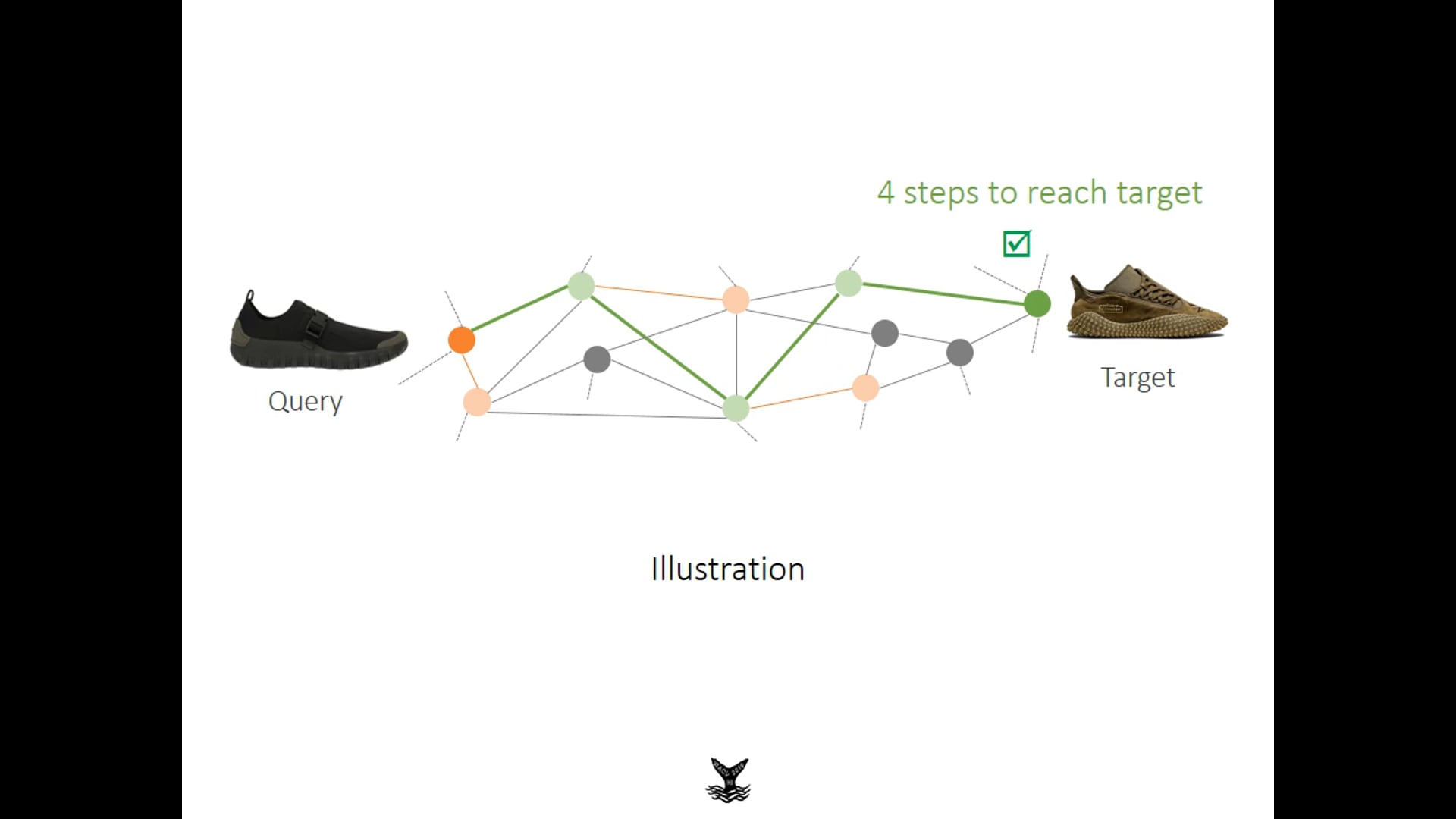
For simplicity, assume that the inventory consists of only a single image per product. We can construct a graph as in Figure 5, where each node is a product. Nodes are connected if they have at least one shared attribute. For example, nodes corresponding to two products from the same brand may be connected. These connections have weights proportional to their similarity, which is based on the distance between their embeddings. Note that these weights depend on the condition of similarity (for example, brand, buckles).

Figure 5. Our setup is also novel in the sense that the entire user feedback process can be simulated, and performance can be evaluated automatically. In fact, this helps us train our deep neural network for reinforcement learning. Given a graph of inventory where each node is an image of a product (for simplicity, assume one image per product), we can randomly sample two nodes, where one is the initial query and the other is the image of the desired product. Our goal is to go from one to the other in as few steps as possible.
Typical approaches requiring such user feedback construct training and validation sets using actual user feedback by crowdsource. This could result in subjective and inconsistent labels. Also, this is an expensive procedure that results in a limitation in the size of the data set. Evaluation of the approach has further complexities related to the repeatability of the experiment. This is easily addressed by simulation. Our goal is to reach the desired product in a minimal number of steps.
Approach
Learn to extract embedding
We train a CSN based on triplets generated from the available attributes in the data set. This creates rich embeddings for each attribute (as in Figure 1). It is important to note that we create triplets based on coarse attribute labels (for example, “are A and B both purple?”) which are easily available instead of the expensive relative attribute labels (for example, “is A more purple than B?”). Figure 6 shows that even coarse labels can produce rich embedding comparable to those achieved by expensive relative attribute labels. We achieve this by using CSN and making some modifications to it (i) restrict mask vector so that all elements add up to 1 (ii) discourage large values for the magnitude of embedding vector (iii) apply global consistency constraints by considering overlap of attributes between pairs. These modifications result in about 3% absolute improvement in accuracy. See our paper for technical details.

Figure 6. The visualization of an embedding using t-SNE for the attribute “closure” on UT-Zappos50k data set. Note that this captures similarity based on shoe style very well even though it was trained to predict “closure.” We were able to learn high-quality embedding with just the binary attributes (for example, “do A and B have the same brand?”) instead of the expensive relative attributes (for example, “is A more purple than B?”). Our modifications to CSN improves absolute accuracy by about 3%.
Learn to navigate
As shown in Figure 4, we use nearest neighbor search (think of visual search) to sample top candidates, and then use reinforcement learning (RL) to rank them and pick the top few (say, two) to be shown to the user. As mentioned in Figure 5, we can simulate the entire procedure for interactive visual search since we can randomly select initial query and final target. RL is very effective for such cases. We use Deep Q-Network (DQN) as in “Playing atari with deep reinforcement learning”, NeurIPS Deep Learning Workshop 2013.
DQN learns to predict the Q-value for a given set of actions from a given state. The Q-value for a given state and action is the maximum expected long-term future reward for that action from that state. For instance, in the game of chess, Q-value could be the probability of winning the game when we make a specific move (the action) from the current configuration of the chess pieces on the board (the state). Note that the short-term reward could be to take out the opponent’s pawn even though this may not necessarily increase the long-term future reward of winning the game. Thus, Q-value is a measure of the quality of action at a given state. Note that it is dependent on both the state as well as the action. The same action may not be optimal at a different state.
In our case, an “action” is selection of an image from the candidate set of images from the sampler. “State” consists of relative embeddings of images with regard to the embedding of the latest query that generated the candidates. As in Figure 7, the best image has the largest estimated Q-value (as indicated by the green checkbox). The DQN consists of three fully connected layers and ReLU as nonlinearity. This is illustrated in Figure 8. As discussed in the previous section, CSN learns a mask that adapts to the condition for similarity. Thus, the sampler can produce candidates per masked embedding. A separate DQN predicts Q-values for the candidate sets from each sampler, as in Figure 9. CSN was trained first, and then DQN was trained using Huber loss (a combination of piecewise linear and squared loss) based on the expected and observed rewards of picking the top images for user feedback. Note that user feedback is simulated. The best image will be the closest to the target image (known during simulation) among all the queries picked so far.

Figure 7. Simplified view of Deep Q-Network showing inputs and outputs. The sampler gives a candidate set of images. The goal of DQN is to pick the top images from this candidate set based on the estimated Q-values. Here, “action” is selection of an image and “state” is defined by the candidate set of images from the sampler. We define the relative embeddings of images with regard to the embedding of the current query image to be the state variables. Also see Figure 8.

Figure 8. Our Deep Q-Network contains three fully connected layers with ReLU as non-linearity. Also refer to Figure 7.

Figure 9. Complete architecture to train the neural networks. This figure shows loss layers for both CSN and DQN. We use ResNet-18 as a backbone for the CSN. The architecture for DQN is shown in Figure 7. The sampler produces nearest neighbors based on the masked embedding. Huber loss is used to train the DQN based on the expected and observed rewards of picking the top images for user feedback.

Figure 10. Sample navigation using our approach. Each row shows the traversal initiated by a query shown on the left. The desired products are highlighted in green boxes at the right. Although not immediately obvious, consecutive products share specific attributes.
See Figure 10 for a qualitative illustration of navigation for various input queries. Every selected image has at least one common attribute with the previous one. The average agreement of human annotators with our simulated approach was about 79%. We observed a reduction in number of steps by 11.5-18.5% when we use our DQN approach, compared to competing hand-engineered rules to rank. The reduction is 17-27% when compared to nearest neighbor. See our paper for technical details.
Summary
We presented a scalable approach for interactive visual search using a combination of CSN (for conditional masked embedding), DQN (no hand-engineered rules), and simulation (train without human-in-the-loop and at scale). Our approach can be easily extended to multimodal data as well as personalization.
Improvements in Embedding
-
No need for expensive relative attribute labels
-
Modified CSN
-
~3% absolute improvement in accuracy (UT Zappos 50K, OSR)
Improvements in Navigation
-
Learn to rank triplets and select candidates using DQN
-
11.5-18.5% reduction in number of steps when compared to competing hand engineered rules to rank
See our paper for technical details, or watch the short video below.
Interactive Visual Search from eBay Newsroom on Vimeo.
Acknowledgements
This is collaborative work with Bryan Plummer who was our summer intern in 2017 and the primary author of our paper.